*Notice: You can download the PDF version of this post*
1 Introduction
When transmitting analog source signals like images and sound over waveform channels, the most common approach is to use separate source and channel coders. Separation of source and channel was proven to be optimal by Shannon [1]. However, the price to pay to achieve near- optimality involve very high encoding/decoding complexity, significant delays, specific design for desired rate/distortion and threshold effect: lack of robustness to small changes in parameters. So in practice, digital systems based on joint source-channel coding (general transformation) may have performance advantages when complexity is constrained. Shannon-Kotel'ikov mapping is a kind of non-linear transformation which can provide both bandwidth reduction and bandwidth expansion.
Shannon-Kotel'ikov mappings are related to channeloptimized vector quantizers as devel- oped by Vaishampayan [2]. As opposed to quantizing the source and thereby creating a discrete set of representation points which are then mapped onto the channel, the Shannon-Kotel'ikov mappings perform either a projection of the source onto a lower dimensional subset (lossy com- pression), or map the source into a higher dimensional space (error control) [3].
2 Simulation
This report performed simulation of 2:1 Bandwidth Reduction with the Archimedes Spiral (as shown in Figure 1) suing MATLAB with methods described in [3]. The simulation is performed for a image signal source as shown in Figure 2(a) and an additive white Gaussian noise (AWGN) channel. A factor-two bandwidth reduction, or compression, is achieved by combining two consecutive samples using a non-linear mapping.
We perform the bandwidth reduction by transmitting a combination of two source samples \( x_1 \) and \( x_2 \) as one channel sample \( y \). This is achieved by first approximating a point in \( R^2 \) to the closest point on the double Archimedes' spirals. The spirals can be described parametrically as,
\[
x_1 = 2 \Delta \frac{\theta}{2 \pi} \cos (\theta),x_2 = 2 \Delta \frac{\theta}{2 \pi} \sin (\theta)
\]
and
\[
x_1 = 2 \Delta \frac{\theta}{2 \pi} \cos (\theta + \pi),x_2 = 2 \Delta \frac{\theta}{2 \pi} \sin (\theta + \pi)
\]
As MATLAB code bellow described, the projection can be achieved by
\[
  \hat \theta = \mathop{argmin}_{\theta}{\{(x_1 \pm \frac{\Delta}{\pi}\theta\sin \theta)^2 + (x_2 - \frac{\Delta}{\pi}\theta\cos \theta)^2\}}
\]
The projected point is still 2-dimension, but can be compressed into 1-dimension \(y\) by
\[
  y = l_{\pm}(r) = \pm \zeta (\frac{\pi}{\Delta})^2 r^2
\]
where \(+\) represents points residing on the blue line and the \(-\) represents points residing on the the red lines in Figure 1. \(r= \frac{\Delta}{\pi}\theta\) and the parameter \(\zeta = \eta \Delta = 0.16 \Delta\) makes this operator an approximation of the length along the spiral. This expression is found by using a nonlinear curve fit on the expression of the true arc length
\[
  l(r)_s = \frac{1}{2}(r\sqrt{1 + (\frac{\pi}{\Delta}r)^2} + \frac{\Delta}{\pi} \sinh^{-1} (\frac{\pi}{\Delta}r))
\]
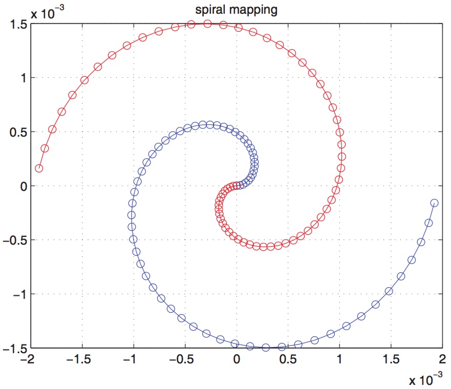 Figure 1. Spiral mapping.
%% spiral curve mapping and transform to 1 dimension
for i=1:test_length
    theta_max = 255*pi/(2*delta_opt(i));
    % max theta of spiral curve calculated from the max radius 255/2
    spiral_length = 0:2:yita*pi^2/delta_opt(i)*(delta_opt(i)/pi*theta_max)^2;
    % array of spiral curve length used to calculate points (x, y) on the curve
    spiral_theta = sqrt(spiral_length./(yita*delta_opt(i)));
    % array of theta calculated from spiral_length
    spiral_x = delta_opt(i)/pi*spiral_theta.*cos(spiral_theta);
    % array of x component of points
    spiral_y = delta_opt(i)/pi*spiral_theta.*sin(spiral_theta);
    % array of y component of points
    for j=1:signal_length
        distance = (spiral_x-source_signal_one(j)).^2+(spiral_y-source_signal_two(j)).^2;
        % distance from given point to spiral curve points
        min_pos = find(distance==min(distance));
        % find the min distance, i.e., mapping given point onto curve
        Y(j, i) = yita*pi^2/delta_opt(i)*(delta_opt(i)/pi*spiral_theta(min_pos))^2;
        % calculate curve length of mapped point for signal transmission
    end
end
As described in [3], when optimizing the spiral mapping, the goal is to find the \(\Delta\) that minimizes the total distortion
\[
  \Delta_{opt} = 2\pi\sigma_x\sqrt[4]{\frac{6 \cdot \eta^2}{CSNR}}
\]
The decoded SNR is given by (as described in [3])
\[
  SNR = \frac{\sqrt{6}}{2\cdot0.16\cdot\pi^2}\sqrt{CSNR}
\]
and the Optimal Performance Theoretically Attainable (OPTA) for the $2:1$ case is given by \(SNR = \sqrt{1+CSNR}\).
White Gaussian noises were added to the signal as passing through the channel, as MATLAB code described bellow.
%% signal pass though noisy channel
for i=1:test_length
    for j=1:signal_length
        Y(j, i) = Y(j, i) + variance_std/CSNR(i)*randn;
        % add white noise of channel
    end
end
Using the inverse operation of \(l(r)\), the received signal can be decoded as described in MATLAB code bellow:
%% decoding signal
for i=1:test_length
    for j=1:signal_length
        theta = sqrt(Y(j, i)/(yita*delta_opt(i)));
        % decode theta from curve length
        decode_signal_one(j, i) = delta_opt(i)/pi*theta*cos(theta);
        % 1D to 2D: x1 component
        decode_signal_two(j, i) = delta_opt(i)/pi*theta*sin(theta);
        % 1D to 2D: x2 component
    end
end
MATLAB code bellow calculated SNRs of simulated result.
%% SNR of simulation
SNR = ones(test_length, 1);
for i=1:test_length
    sample_image = decode_signal_one(:, i);
    sample_image = reshape(sample_image, row, column)+(255/2.0);
    error = sample_image - double(image);
    SNR(i) = 10*log10(signal_power/mean(mean(abs(error.^2))));
end
3 Results and Discussion
The results of 2:1 Bandwidth Reduction with the Archimedes Spiral simulation are shown in Figure 2 and Figure 3. Figure 2 (a), (b), (c) and (d) are the original image, reconstructed image with CSNR = 30db, 16dB and 4dB separately.
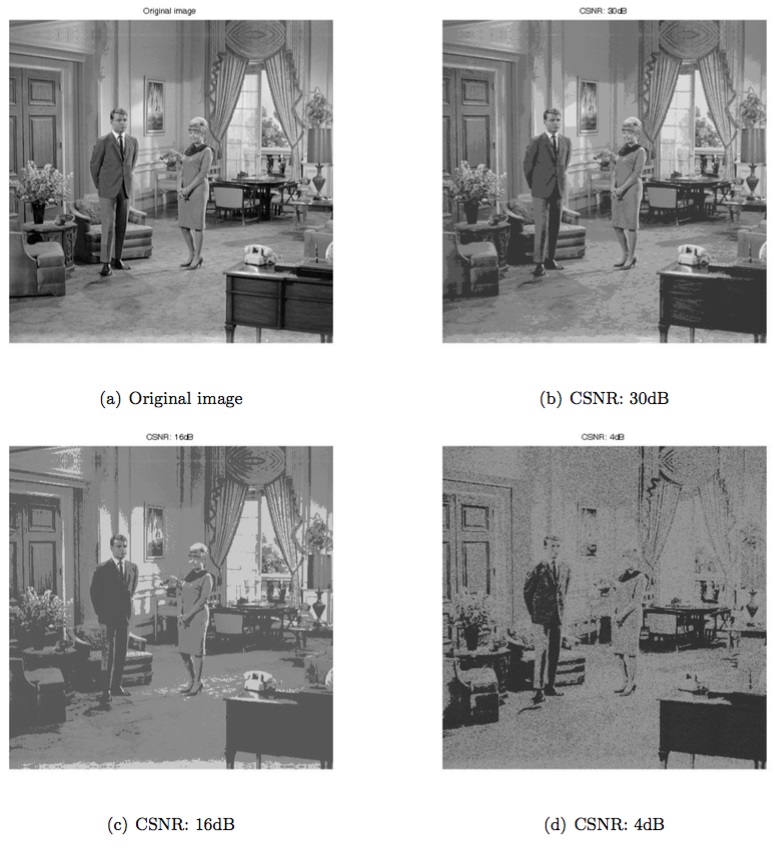 Figure 2. (a) Original image (b) Reconstructed image with CSNR = 30dB (c)
Reconstructed image with CSNR = 16dB (d) Reconstructed image with CSNR = 4dB.
Figure 2. (a) Original image (b) Reconstructed image with CSNR = 30dB (c)
Reconstructed image with CSNR = 16dB (d) Reconstructed image with CSNR = 4dB.
As calculated, the system has an SNR only \(\sqrt{6}/\pi = 1.1\) dB away from OPTA, which is shown clearly in the Figure 3. Limited by methods used in the MATLAB simulation, the performance is different from the SNR calculated, better or worse. As we can see, as CSNR increase from 20 to 30, the simulation results were narrowly worse than the results of calculation, which may be limited by some method used in the simulation. Further research should be focusing on this.
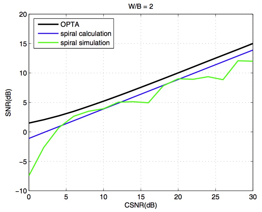 Figure 3. Optimal performance theoretically attainable (OPTA).
References
[1] C. E. Shannon, A mathematical theory of communication. The Bell System Technical J., vol. 27, pp. 379-423, 1948
[2] V. A. Vaishampayan. Combined source-channel coding for bandlimited waveform channels. Ph.D. dissertation. University of Maryland. 1989.
[3] Fredrik Hekland, Pal Anders Floor and Tor A. Ramstad. Shannon-Kotel'nikov Mappings in Joint Source-Channel Coding. IEEE TRANSACTIONS ON COMMUNICATIONS. VOL. 57, NO. 1, JANUARY 2009.